Chapter 1: OLS Regression Basics

1.1 Introduction

The basic linear regression aims to establish a relationship between a dependent variable and one or more independent variables. Thus, one assumes that the value of the dependent variable is a function of the value(s) of the independent variable(s): \(y_{i} = f\left( x_{i,1},x_{i,2},\ldots,\ x_{i,n} \right)\). In practice, this relationship must be estimated. A “simple linear regression” involves only one independent variable. A “multiple regression” involves more than one independent variable. The dependent variable is also called the regressand. The independent variables are also called regressors.

A linear regression tautologically assumes this relationship is linear. In this case, one constructs the “line of best fit”, which is the best linear approximation of the relationship between the value of the dependent variable and the values of the independent variables. Ordinarily, in a linear regression, the mean is assumed to be a linear function of the regressors.

In practice, there are several steps in a regression analysis. These are often mechanical. However, it is important to understand the background behind the analysis so that you can determine when, or whether, there is an error.

1.2 Technical details

Assume there are \(n\) individual units. For example you might want to examine a set of \(n\) firms. If this were all the firms in the S&P 500, then \(n = 500\). Denote each individual firm with the subscript i. Thus, there are \(i = \left\{ 1,\ldots,n \right\}\) firms. For each of these observations, we want to model a variable of interest (the regressand, or independent variable). For example, we might want to model the factors that influence firms’ earnings. For each observation, we can also observe a set of factors we believe could influence the regressand. For example, for the firms’ earnings, this could be capital expenditure, R&D etc. If we look at the set of 500 firms at one point in time (i.e., the earnings in 2020), then we have a cross-sectional regression. If we look at the earnings for multiple years, we have a panel regression (i.e., multiple observations for each firm).

The linear regression is represented as follows:

Where, \(y_{i}\) represents the value of the dependent variable for unit \(i\) (i.e., earnings for one of the firms in the S&P 500), \(x_{i}^{(j)}\) represents the \(j^{th}\) regressor for firm \(i\), \(\theta^{(j)}\) is the regression coefficient, and \(\alpha\) is the intercept term. Here, \(\varepsilon_{i}\) represents the “error” term. This arises because we have forced there to be a linear relationship between the regressand and the regressor. The error term represents the difference between the observed value of \(y_{i}\) and the value predicted in the linear model. By definition, the error term is zero on average. That is \(E\left( \varepsilon_{i} \right) = 0\).

The regression can also be expressed using matrix notation. Here, \(y_{i} = \mathbf{x}_{i}^{T}\mathbf{\theta}\), where \(\mathbf{x}_{i}^{T}\) represents the vector of regressors for firm \(i\). So, if there are five regressors, then \(\mathbf{x}_{i}\) is a 5 x 1 vector, and \(\mathbf{x}_{i}^{T}\) is its transpose (which is a 1 x 5 vector). Here, \(\mathbf{\theta}\) is the 5 x 1 vector of regressor coefficients. It is also possible to create a regressand vector, which puts all the observations into a single vector. In this case, the regression is expressed as \(\mathbf{y = X\theta}\), where \(\mathbf{y}\) is the regressand vector and \(\mathbf{X}\) regressor matrix. The vectors are then:

Where here:

• \(\mathbf{y}\) is a \(n \times 1\) vector, representing the regressand.

• \(\mathbf{x}\) is an\((m + 1) \times 1\) vector representing the regressors, and including an initial “1” value to incorporate the intercept term.

• \(\mathbf{\theta}\) is a \((m + 1) \times 1\) vector representing the regression coefficients.

• \(\mathbf{X}\) is a \(n \times (m + 1)\) matrix , which is effectively a stacked set of regressor vectors.

1.3 What are the regression assumptions?

The linear regression makes several assumptions. The regression analyst should determine whether these assumptions hold. And, if relevant, take steps to mitigate any specification issues that arise. The assumptions are as follows:

Linearity: The linearity assumption is simply that the relationship between \(y\) and \(x\) is linear. This is tautologically evident from the regression specification. Note, however, that is possible to transform variables that otherwise have a non-linear relationship so that the transformations are linear. For example, where applicable, one can take logs of regressors or regressands. The equation can also include polynomial terms if the regressand is a polynomial function of the regressors. For example, if \(y_{i}\) is a quadratic function of \(x_{i}\), then the regression can include both \(x_{i}\) and the squared term \(x_{i}^{2}\). Then, the linear regression would become \(y_{i} = \alpha + x_{i}\beta^{(1)} + x_{i}^{2}\beta^{(2)} + \varepsilon_{i}\).

Homoscedasticity (constant variance): Homoscedasticity stipulates that the variance of the error term is constant for any value of the regressors \(x\). The opposite of homoscedasticity is heteroscedasticity (which is where the error variance differs across observations). This is violated if particular groups of observations have different error variances. For example, if the dataset contains data for firms in several industries, these industries might have data clustering. Here, the error variance might differ between industries. This can be addressed through a combination of clustered standard errors, heteroscedasticity consistent standard errors, or, where relevant, including additional or more appropriate regressors.

The homoscedasticity assumption can be expressed mathematically as \(E\left\lbrack \varepsilon_{i}^{2} \middle| \mathbf{X} \right\rbrack = \sigma^{2}\), where \(\sigma^{2}\) is the same constant variance for each observation.

Independent errors: This assumption is that errors are not correlated with each other. Mathematically, this means \(E\left\lbrack \varepsilon_{i}\varepsilon_{j} \middle| \mathbf{X} \right\rbrack = 0\) for all \(i \neq j\). This also implies a lack of autocorrelation. This might be violated in time series data where there is a time series correlation in the data.

Normality: This assumption is that the errors are normally distributed. Note that the regression model can still be valid notwithstanding non-normal errors. This assumption thus implies that the errors are normally distributed with mean zero and variance \(\sigma^{2}\).

1.4 How to find (or derive) the coefficient values

The regression values are the coefficients that minimize the errors. Ordinary least squares (OLS) regression thus aims to minimize the squared errors: \(\mathbf{\varepsilon}^{\mathbf{2}}\). The focus is on the squared error because some errors are negative and some are positive. Thus, if they are not squared, the negatives and positives could cancel out, giving a false impression of the regression’s accuracy. Let us walk through the derivation:

First, note that the error term is \(\mathbf{\varepsilon = y - X\theta}\). The error term is a \(n \times 1\) vector. Thus, to get the sum of squared errors, we need \(\mathbf{\varepsilon}^{\mathbf{T}}\mathbf{\varepsilon}\) (i.e., a \(1 \times n\) vector multiplied with a \(n \times 1\) vector). Therefore, we obtain the following relationship:

We can apply the transpose to the first set of parentheses to obtain \(\left( \mathbf{y - X\theta} \right)^{T} = \mathbf{y}^{T} - \mathbf{\theta}^{T}\mathbf{X}^{T}\) (due to how transpose rules work in matrix algebra). Therefore, \(\mathbf{\varepsilon}^{\mathbf{T}}\mathbf{\varepsilon =}\left( \mathbf{y}^{T} - \mathbf{\theta}^{T}\mathbf{X}^{T} \right)\left( \mathbf{y - X\theta} \right)\). We can then multiply through and obtain:

We can simplify this further. Notice that \(\mathbf{y}^{T}\mathbf{X\theta}\) is a 1 x 1 matrix. This is because \(\mathbf{y}^{T}\) is \(1 \times n\), \(\mathbf{X}\) is \(n \times m\), and \(\mathbf{\theta}\) is \(m \times 1\). Further, \(\mathbf{\theta}^{T}\mathbf{X}^{T}\mathbf{y =}\left( \mathbf{y}^{T}\mathbf{X\theta} \right)^{T}\), which is also a 1 x 1 matrix. Therefore, \(\mathbf{y}^{T}\mathbf{X\theta =}\left( \mathbf{y}^{T}\mathbf{X\theta} \right)^{T}\). Therefore, \(\mathbf{y}^{T}\mathbf{X\theta =}\mathbf{\theta}^{T}\mathbf{X}^{T}\mathbf{y}\). Therefore, we can simplify the expression for \(\mathbf{\varepsilon}^{\mathbf{T}}\mathbf{\varepsilon}\) to be:

Now, we want to minimize \(\mathbf{\varepsilon}^{\mathbf{T}}\mathbf{\varepsilon}\) by choosing the appropriate coefficient values. Therefore, we differentiate \(\mathbf{\varepsilon}^{\mathbf{T}}\mathbf{\varepsilon}\) with respect to \(\mathbf{\theta}\) and set the derivative to zero to find the minimum. One can also obtain the second derivative to verify that the curve is concave up. The first derivative is thus:

This yields:

Set the derivative equal to zero and solve for \(\mathbf{\theta}\) to obtain:

1.5 How to know if the coefficients are statistically significant?

A researcher must first determine whether a coefficient is statistically significant. This involves hypothesis testing to determine whether the coefficient is statistically significantly different from zero (or another hypothesized value).

The first step is to obtain and understand the standard error for the coefficient. This is a representation of its variability. Most statistical packages produce this automatically. The derivation starts with the basic definition for variance (i.e., the variance of x is (x-E(x))²_. Therefore:

Where, \(E(\mathbf{\theta)}\) denotes the true population value for the coefficients. Given that we know that \(\mathbf{\theta} = \left( \mathbf{X}^{T}\mathbf{X} \right)^{- 1}\mathbf{X}^{T}\mathbf{y}\), we can expand it as follows:

But, we also know that \(\mathbf{y = X\theta + \varepsilon}\). Therefore, we get:

Therefore, we can note that \(\mathbf{X}\) is non-stochastic, and we can obtain,

Thus, assuming homoscedasticity, we know that \(E\left\lbrack \mathbf{\varepsilon}\mathbf{\varepsilon}^{T}|\mathbf{X} \right\rbrack = \sigma\mathbf{I}\), where \(\sigma\) is the constant variance of the errors and \(\mathbf{I}\) is the identity matrix. We can also collect the various \(\mathbf{X}\) terms. Therefore, we obtain:

In practice, statistical packages report the following: (1) coefficient standard error, (2) coefficient t-statistic, and (3) coefficient p-value. The standard error is a useful input to calculate the t-statistics, which in turn allow one to obtain the p-value. Here, the t-statistic is:

Where, \(\theta\) denotes the coefficient from the regression output, \(\theta_{0}\) is the hypothesized coefficient value against which the coefficient is tested for significance, and \(s.e.(\theta)\) is the standard error of the regression coefficient. By default, regression packages test whether the coefficient is statistically significantly different from zero. However, an analyst can test against other hypothesized values. For example, \(\theta_{0}\) might be set to one when analyzing whether a firm’s stock beta differs from the market beta of one.

The p-value is a measure of statistical significance. A lower p-value connotes higher confidence that the coefficient is statistically different from the null. Technically, for a two-sided hypothesis test, the p-value is the probability that you would observe a coefficient value at least as extreme as the one observed if the null hypothesis about the coefficient is true.

In simple terms: Suppose your null hypothesis is the coefficient is zero. But, you observe a coefficient value of \(\theta'\). Then, the p-value is the probability that you would observe a coefficient of \(\theta'\) if it were in fact true that the coefficients should be zero on average. A lower p-value signifies greater confidence that the coefficient differs from zero as it would connote a lower probability of observing a coefficient that extreme if the null were true.

There are some general rules for interpreting p-values. The general rule of thumb is that a p-value of less than 0.05 connotes reasonable statistical confidence that the coefficient is not equal to zero (assuming the null is zero). A p-value less than 0.01 signifies a high degree of statistical confidence. A p-value between 0.05 and 0.1 signifies an acceptable level of statistical confidence. It is important to note that these are general rules and all cases should be considered based on their own circumstances.

1.6 Regression Performance Metrics

It is important to evaluate the regression’s efficacy. There are several ways to do this. The metrics are not mutually exclusive and they provide different information. Further, when assessing what a “good value” is for a metric, it is important to compare the value you obtain to what is standard in the literature for your project. The key performance metrics are as follows:

Mean squared error (MSE): The MSE is the average regression error term. It tells you how far the predicted value is from the actual value on average. The error term is squared in order to avoid negative errors cancelling out positive errors, which could make an otherwise error-prone model appear relatively accurate. The MSE has some advantages over the mean absolute error (MAE): it is differentiable and penalizes large errors, which can be beneficial. The calculation is as follows:

Where, \(y_{i}\) is the observed value of the regressand, and \(\widehat{y}\) is the value that the regression model predicts. The term \(\widehat{y}\) is sometimes denoted as \(E\left( y_{i} \right)\).

Root mean squared error (RMSE): The RMSE is the square root of the MSE. This might be preferred if there are large error values and the MSE appears to over-emphasize them. Thus, \(RMSE = \sqrt{MSE}\).

Mean absolute error (MAE): The mean absolute error is the average absolute error for the regression terms. It penalizes large errors less than does MSE. This is because the MSE squares the error term, causing it to emphasize those large errors. The disadvantage of the MAE is that differentiation is less straightforward. The MAE is thus:

R squared (\(\mathbf{R}^{\mathbf{2}}\)): The R-squared is a measure of “goodness of fit”. It aims to determine how well the regression line fits the data. A higher R-squared is generally better. However, a higher R-squared can tautologically arise if the model includes more, but marginally meaningful, variables. The adjusted R-squared (see below) resolves this. In short, the R-squared looks at how much of the total variance in the dependent variable the model is capable of explaining. That is:

The numerator is the model variance. This is the MSE defined above. The total variance in the dependent is the mean squared deviation of the observed value from the average value. That is, it is much like a variance measure for the dependent variable. It is thus, \(\frac{1}{n}{\sum_{i = 1}^{N}\left( y_{i} - \overline{y} \right)}^{2}\). Therefore, the R-squared can be expressed as:

Adjusted R squared: The Adjusted R-squared penalizes the R squared for the number of regressors. The adjusted R squared can be no larger than the R squared. In general, researchers focus on the adjusted R squared rather than the plain R squared. The precise calculation is as follows:

Where \(n\) is the number of observations, \(k\) is the number of regressors, and \(R^{2}\) denotes the ordinary R squared.

1.7 Example: interpreting regression output

Let us apply some of what we have learned to an example. Suppose we want to analyze the factors that influence car prices. Let us take a somewhat randomly determined set of 74 make/model prices, which are available via Stata (when using Stata, this dataset is available using the command “sysuse auto”). The specifics of the data are largely irrelevant to our discussion.

We can then estimate a regression where we analyze whether several variables influence car prices. This regression uses a sub-set of the available variables and is for illustration purposes. The set of regressors is not exhaustive. Here, we run a regression where the dependent variable is the natural log of the car’s price. The regressors are its miles per gallon (mpg), the natural log of its weight (lnweight) and an indicator variable for whether the car is foreign or domestic, in order to broadly capture factors such as transportation costs and import duties (foreign). This is a standard OLS model. The baseline regression command in stata is “reg lnprice mpg lnweight foreign”. The regression equation is as follows:

Where, the variables are as described above, the \(\alpha\) term represents the regression intercept, the \(\beta\) terms represent the regression coefficients, and \(\varepsilon\) represents the residual or error term.

When we run the regression we obtain the regression output from Stata. This regression output is similar across statistical packages. However, the layout can vary between packages. Let us interpret the interesting parts of this regression output.

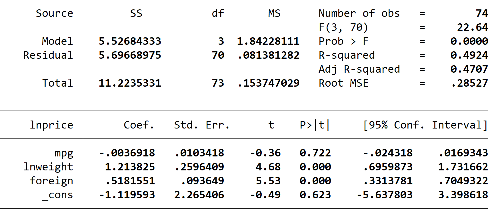
We can start with basic regression information and performance. Here, the R-squared and Adjusted R-squared are similar at approximately 49% and 47%, respectively. This indicates that around 49% of the variation in the dependent variable can be explained by variation in the regressors. In general terms, this is a strong result for data such as this. While the MSE and the Sum of Squared numbers are interesting, they are primarily relevant when used in other measures, such as the R-squared.

We can next analyze the coefficients. The F-statistic indicates that the coefficients in general are different from zero. The F-statistic tests the null that the regression coefficients are jointly zero. Another way to think about it is it tests whether the regression with regressors performs better at explaining the dependent variable than does a regression with no regressors. Here, the F-statistic is highly statistically significant, as indicated by its p-value of zero. However, this only analyzes the coefficients in general. It does not tell us whether any individual coefficient is meaningful.

Some of the coefficients are individually significant. First, the mpg coefficient is not statistically significant. The coefficient is near to zero. The p-value is 0.722. This implies that the coefficient is not statistically meaningful. Second, lnweight is statistically significant. The coefficient is 1.21 and the p-value is zero. This implies that it is highly likely that the coefficient is statistically distinguishable from zero. Third, the foreign car indicator is 0.518 and has a p-value of zero. This implies that foreign cars have higher prices in our sample.

We can now interpret the regression coefficients. Let us ignore mpg for the moment; it is not statistically significant. The foreign car indicator is the easiest to interpret. It implies that foreign cars in our sample have a 0.518 increase in lnprice. The question is what this means. Because we are looking at log prices, it means that while a domestic car price might be ln(x) a foreign car price is ln(x+0.518). Thus, in terms of percentage change, the percentage difference is ln(x+0.518)/ln(x). To interpret this we need to consider the average value of lnprice for domestic cars (i.e., the x) in our formula: this is 8.62. Thus, foreign cars are around 6% more expensive than are domestic cars.

The coefficient on the “weight” coefficient indicates that prices increase with weight. Here, the coefficient is 1.214. The standard deviation of lnweight is 0.26634. Therefore, we can say that a one standard deviation increase in lnweight is associated with a 1.214 x 0.26634 = 0.323 increase in lnprice. The average value for lnprice is 8.64 (including both foreign and domestic cars). Therefore, the percentage impact of a one standard deviation increase in weight is a 3.7% increase in price.